

This guide will teach you the process of exporting data from a relational database (MySQL) and...
This guide will teach you the process of exporting data from a relational database (MySQL) and importing it into a graph database (Neo4j). You will learn how to take data from the relational system and to the graph by translating the schema and using Apache Hop as import tools. This Tutorial uses a specific data set, but the principles in this tutorial can be applied and reused with any data domain.
This guide was inspired by the original Neo4j Northwind tutorial. We've borrowed parts of the original post for context and completeness. The actual data loading is done with the Neo4j functionality in Apache Hop.
In this guide, we'll walk through the process with the Graph Output transform. This transform allows you to (re-)use a graph model based on metadata to load data from your relational database directly to Neo4j.
Check our previous post on how to do this using the Neo4j Output transform. The result of both posts is the same, but the process is a little different. We'll go into the difference between these two in a later post.
Prerequisites:
- You should have a basic understanding of the property graph model and know how to model data as a graph.
This tutorial can be followed using an AuraDB instance and Apache Hop:
Neo4j Aura
Neo4j Aura is free. Start on AuraDB
Alternatively, you can:
- Start a Blank Neo4j Sandbox
- Download and install Neo4j Desktop.
Apache Hop
Apache Hop is a data engineering and data orchestration platform that allows data engineers and data developers to visually design workflows and data pipelines to build powerful solutions.
As an Apache project, Apache Hop is also free. Get started with Apache Hop.
About the Data Set
In this guide, we will be using the Northwind dataset, an often-used SQL dataset. This data depicts a product sale system - storing and tracking customers, products, customer orders, warehouse stock, shipping, suppliers, and even employees and their sales territories. Although the Northwind dataset is often used to demonstrate SQL and relational databases, the data also can be structured as a graph.
An entity-relationship diagram (ERD) of the Northwind dataset is shown below.
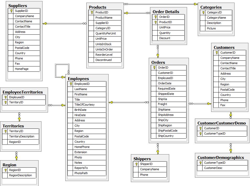
First, this is a rather large and detailed model. We can scale this down a bit for our example and choose the entities that are most critical for our graph - in other words, those that might benefit most from seeing the connections. For our use case, we really want to optimize the relationships with orders - what products were involved (with the categories and suppliers for those products), which employees worked on them, and those employees' managers.
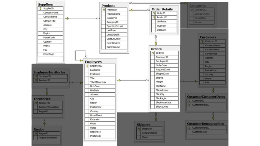
Using these business requirements, we can narrow our model down to these essential entities.
Developing a Graph Model
The first thing you will need to do to get data from a relational database into a graph is to translate the relational data model into a graph data model. Determining how you want to structure tables and rows as nodes and relationships may vary depending on what is most important to your business needs.
For more information on adapting your graph model to different scenarios, check out the modeling designs guide.
When deriving a graph model from a relational model, you should keep a couple of general guidelines in mind.
- A row is a node.
- A table name is a label name.
- A join or foreign key is a relationship.
With these principles in mind, we can map our relational model to a graph with the following steps:
Rows to Nodes, Table names to Labels
- Each row on our
Orderstable becomes a node in our graph withOrderas the label. - Each row on our
Productstable becomes a node withProductas the label. - Each row on our
Supplierstable becomes a node withSupplieras the label. - Each row on our
Employeestable becomes a node withEmployeeas the label.
Joins to relationships
- Join between
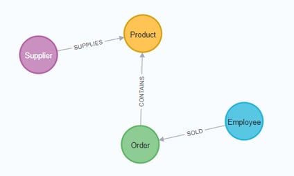
SuppliersandProductsbecomes a relationship namedSUPPLIES(where supplier supplies product). - Join between
EmployeesandOrdersbecomes a relationship namedSOLD(where employee sold an order). - Join with join table (
Order Details) betweenOrdersandProductsbecomes a relationship namedCONTAINSwith properties ofunitPrice,quantity, anddiscount(where order contains a product).
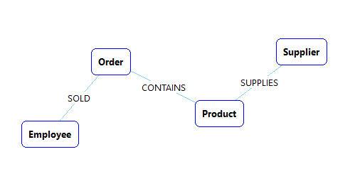
If we draw our translation out on the whiteboard, we have this graph data model.
Now, we can, of course, decide that we want to include the rest of the entities from our relational model, but for now, we will keep to this smaller graph model.
How does the Graph Model Differ from the Relational Model?
- There are no nulls. Non-existing value entries (properties) are just not present.
- It describes the relationships in more detail. For example, we know that an employee SOLD an order rather than having a foreign key relationship between the Orders and Employees tables. We could also choose to add more metadata about that relationship, should we wish.
- Either model can be more normalized. For example, addresses have been denormalized in several of the tables but could have been in a separate table. In a future version of our graph model, we might also choose to separate addresses from the
Order(orSupplierorEmployee) entities and create separateAddressnodes.
Exporting and importing data to Neo4j
With the Neo4j tools
With Neo4j you can follow the next two steps to extract your data from your relational database and load it into your Neo4j database:
1. Exporting Relational Tables to CSV
If you are working with another data domain, you will need to take the data from the relational tables and put it in another format for loading to the graph. A common format that many systems can handle is a flat file of comma-separated values (CSV).
Here is an example script to export the northwind data into CSV files.
export_csv.sql
| COPY (SELECT * FROM customers) TO '/tmp/customers.csv' WITH CSV header; COPY (SELECT * FROM suppliers) TO '/tmp/suppliers.csv' WITH CSV header; COPY (SELECT * FROM products) TO '/tmp/products.csv' WITH CSV header; COPY (SELECT * FROM employees) TO '/tmp/employees.csv' WITH CSV header; COPY (SELECT * FROM categories) TO '/tmp/categories.csv' WITH CSV header; COPY (SELECT * FROM orders LEFT OUTER JOIN order_details ON order_details.OrderID = orders.OrderID) TO '/tmp/orders.csv' WITH CSV header; |
2. Importing the Data using Cypher
You can use Cypher’s LOAD CSV command to transform the contents of the CSV file into a graph structure.
When you use LOAD CSV to create nodes and relationships in the database, you have two options for where the CSV files reside:
- In the import folder for the Neo4j instance that you can manage.
- From a publicly-available location such as an S3 bucket or a GitHub location. You must use this option if you are using Neo4j AuraDB or Neo4j Sandbox.
You use Cypher’s LOAD CSV statement to read each file and add Cypher clauses after it to take the row/column data and transform it into the graph.
Next, you will execute Cypher code to:
- Load the nodes from the CSV files.
- Create the indexes and constraints for the data in the graph.
- Create the relationships between the nodes.
The full process requires a number of manual steps to load your CSV files to Neo4j using LOAD CSV and Cypher. Check the Tutorial: Import Relational Data Into Neo4j to see how that works. Let's see how this can be done with Apache Hop.
With Apache Hop
With Apache Hop, you can do both steps with some simple pipelines/workflows, including the creation of the indexes. This may sound a bit more complex on the query and model side, but the process is a lot simpler. What's even more important is that the process of running Hop workflows and pipelines makes it possible to manage this as part of your entire process life cycle.
Step 1: Create the Graph Model
Apache Hop includes the creation of a Neo4j Graph Model as a metadata object. A graph model in Apache Hop describes (part of) a graph by allowing you to define nodes with their properties, and the relationships that connect these nodes. You can then use such a Graph Model to map input fields to properties in the Neo4j Graph Output transform.
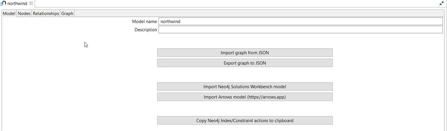
We configure the Northwind graph model as follows:
In the first tab, we specify the model name: Northwind.

Nodes
To create the nodes, we add the Labels: Employee in this case, and the Properties: id, title, last_name, first_name. We also specify the primary key: id.
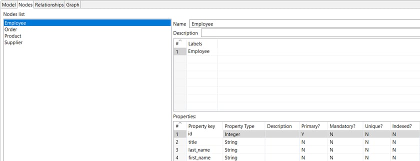

For now, we have all the Northwind nodes:
OrderProductSupplierEmployee
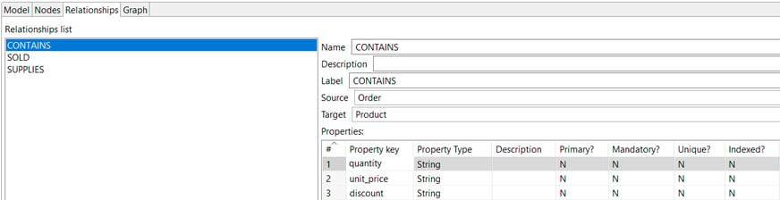
Relationships
After creating all the nodes, we configure all the relationships by specifying the fields:
- Name:
CONTAINS Label:CONTAINSSource:Order, specify the origin node of the relationship.- Target:
Product, specify the target node of the relationship. - Properties:
quantityunit_pricediscount
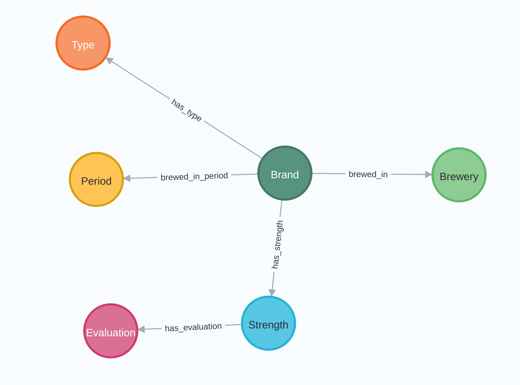
The Graph Model
In the Graph tab, you can visually check the model you just created:
Step 2: loading the data to Neo4j
Now, we are ready to import the data to the Neo4j database. We use a Hop pipeline with a Table Input and a Neo4j Graph Output transform:
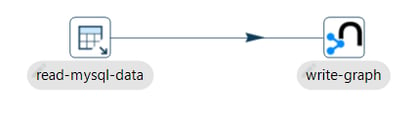

The Table Input transform read the data from the Northwind database using a MySQL connection:
SQL
SELECT s.id AS supplier_id,
s.company AS company,
p.id AS product_id,
p.product_name,
p.category,
o.id AS order_id,
o.ship_name,
e.id AS employee_id,
e.job_title AS title,
e.first_name,
e.last_name,
od.quantity,
od.unit_price,
od.discount
FROM northwind.suppliers s
JOIN northwind.products p ON s.id = p.supplier_ids
JOIN northwind.order_details od ON p.id = od.product_id
JOIN northwind.orders o ON od.order_id = o.id
JOIN northwind.employees e ON o.employee_id = e.id
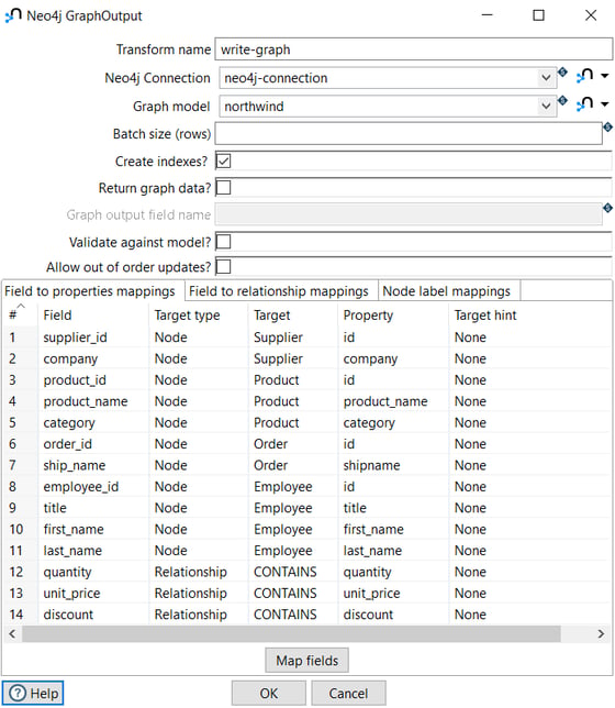
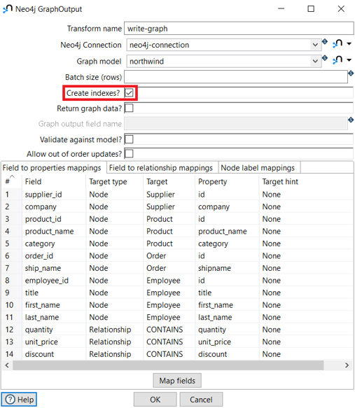
The Neo4j Graph Output transform loads the data into the Neo4j Northwind database using the created Neo4j Graph Model as reference. In this transform, we'll map the available fields to the nodes and relationships we created in the model.


- Transform name:
write-graph, the name for this transform in the pipeline. - Neo4j Connection:
neo4j-connection, select the Neo4j connection to write the graph to. - Graph model:
northwind, select the graph model we created. - Fields: to map the input-output fields, you can use the Map fields option.
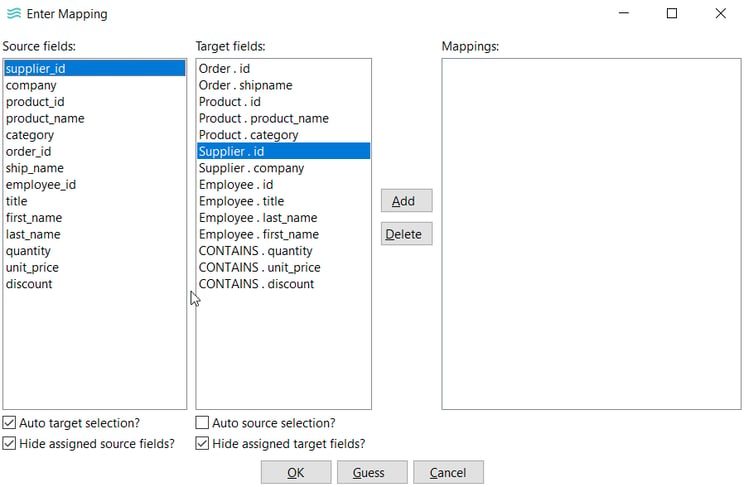

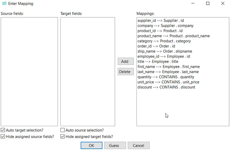
You can use select the fields and hit the Add option or use the Guess option to generate all the mappings.
The mapping looks like this in the image:
 After clicking
 OK you can the fields mapping:
Run your pipeline to populate your Neo4j Northwind database. Check our 5 minute guide on how to load data to Neo4j with Apache Hop for more details.
Explore your newly loaded graph
After your pipeline ran successfully, you have a graph database with your Northwind data. Let's walk through what you just created.
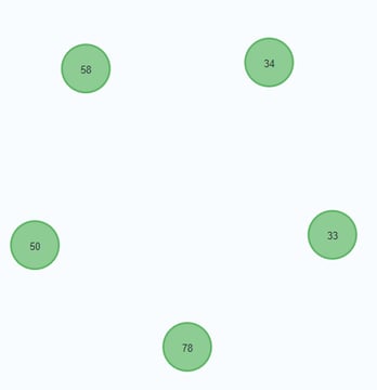
Order nodes
The execution of the pipeline creates 40 Order nodes in the database.
You can view some of the Order nodes in the database by executing this code:
Cypher:
MATCH (o:Order) RETURN o LIMIT 5;
The graph view is:

The table view contains these values for the node properties:
| o |
|---|
|
|
|
|
|
|
|
|
|
|
You might notice that you don’t have to import all of the field columns in the orders table. With your statements, you can choose which properties are needed on a node, which can be left out, and which might need to be imported to another node type or relationship.
Product nodes
The execution of the pipeline creates 24 Product nodes in the database.
You can view some of the nodes in the database by executing this code:
Cypher:
MATCH (p:Product) RETURN p LIMIT 5;
The graph view is:
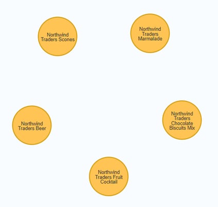

The table view contains these values for the node properties:
| p |
{"id":17,"category":"Canned Fruit & Vegetables","product_name":"Northwind
2Traders Fruit Cocktail"}
|
{"id":19,"category":"Baked Goods & Mixes","product_name":"Northwind
Traders Chocolate Biscuits Mix"} |
{"id":20,"category":"Jams, Preserves","product_name":"Northwind
Traders Marmalade"} |
{"id":21,"category":"Baked Goods & Mixes","product_name":"Northwind
Traders Scones"} |
{"id":34,"category":"Beverages","product_name":"Northwind Traders Beer"} |
Supplier nodes
The execution of the pipeline creates 9 Supplier nodes in the database.
You can view some of the nodes in the database by executing this code:
Cypher:
MATCH (s:Supplier) RETURN s LIMIT 5;
The graph view is:
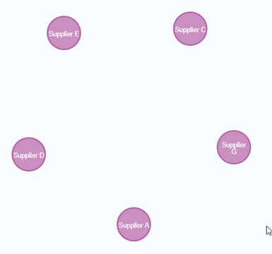

The table view contains these values for the node properties:
| s |
|---|
|
|
|
|
|
|
|
|
|
|
Employee nodes
The execution of the pipeline creates 8 Employee nodes in the database.
You can view some of the nodes in the database by executing this code:
Cypher:
MATCH (e:Employee) RETURN e LIMIT 5;
The graph view is:
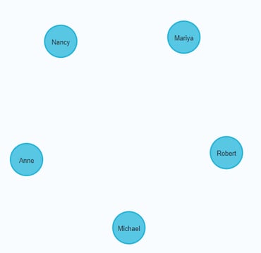

The table view contains these values for the node properties:
| e |
|---|
{"last_name":"Neipper","id":6,"title":"Sales Representative","first_name":"Michael"} |
{"last_name":"Zare","id":7,"title":"Sales Representative","first_name":"Robert"} |
{"last_name":"Sergienko","id":4,"title":"Sales Representative","first_name":"Mariya"} |
{"last_name":"Freehafer","id":1,"title":"Sales Representative","first_name":"Nancy"} |
{"last_name":"Hellung-Larsen","id":9,"title":"Sales Representative","first_name":"Anne"} |
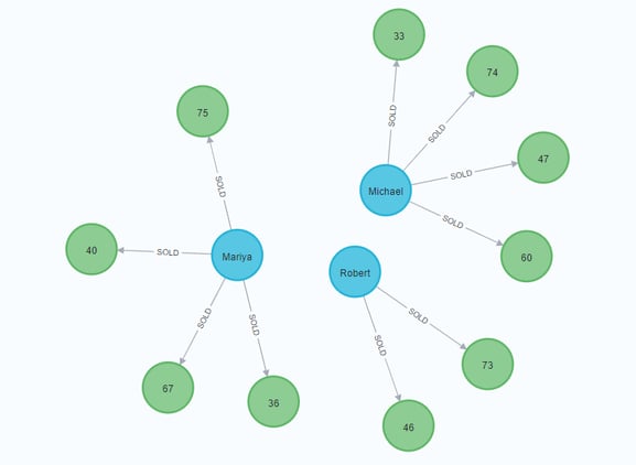
Relationships between Orders and Employees
The execution of the pipeline creates 40 SOLD relationships in the graph database.
You can view some of them by executing this code:
Cypher:
MATCH (o:Order)-[]-(e:Employee)
RETURN o, e LIMIT 10;
Your graph view should look something like this:

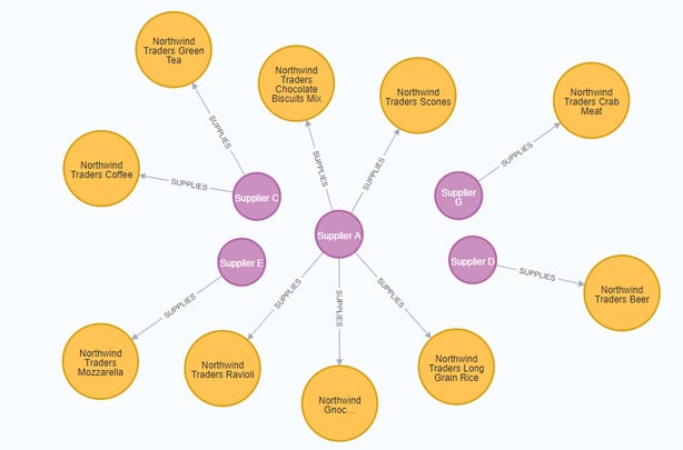
Relationships between Supplier and Product
The execution of the pipeline creates 24 SUPPLIES relationships in the graph database.
You can view some of them by executing this code:
Cypher:
MATCH (s:Supplier)-[]-(p:Product)
RETURN s, p LIMIT 10;
Your graph view should look something like this:
Relationships between Order and Product
The execution of the pipeline creates 58 CONTAINS relationships in the graph database.
You can view some of them by executing this code:
Cypher:
MATCH (o:Order)-[]-(p:Product)
RETURN o, p LIMIT 10;
Your graph view should look something like this:
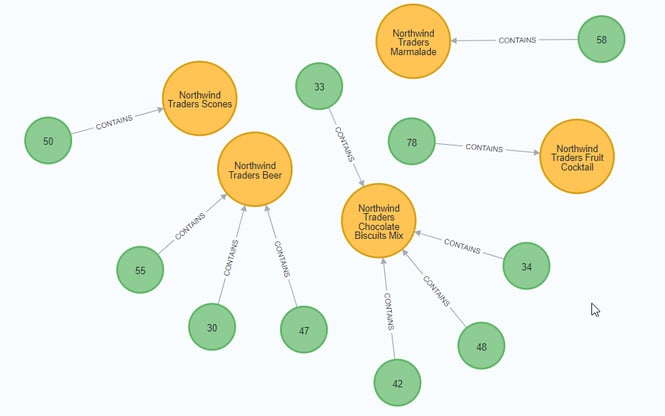

Notice that this relationship includes the properties: quantity, unit_price, and discount.
Example:
{
"identity": 34,
"start": 1,
"end": 0,
"type": "CONTAINS",
"properties": {
"discount": "0.0",
"quantity": "40.0",
"unit_price": "39.0"
}
}
Creating the indexes for the data in the graph
With Cypher, after the nodes are created, you need to create the relationships between them. Importing the relationships will mean looking up the nodes you just created and adding a relationship between those existing entities. To ensure the lookup of nodes is optimized, you will create indexes for any node properties used in the lookups (often the id or another unique value).
To do so you need to execute this code block:
Cypher:
CREATE INDEX product_id FOR (p:Product) ON (p.productID);
CREATE INDEX product_name FOR (p:Product) ON (p.productName);
CREATE INDEX supplier_id FOR (s:Supplier) ON (s.supplierID);
CREATE INDEX employee_id FOR (e:Employee) ON (e.employeeID);
CREATE INDEX category_id FOR (c:Category) ON (c.categoryID);
With Apache Hop, you can include the indexes creation in the pipeline execution by selecting the Create indexes option in the Neo4j Graph Output transform:
Alternatively, you can use the Neo4j Constraint and Neo4j Index actions to manage your Neo4j indexes and other constraints in a more controlled way.

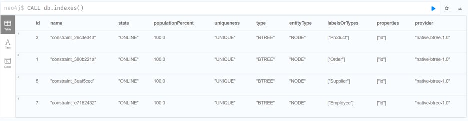
Cypher:
CALL db.indexes();

You should see these indexes in the database:
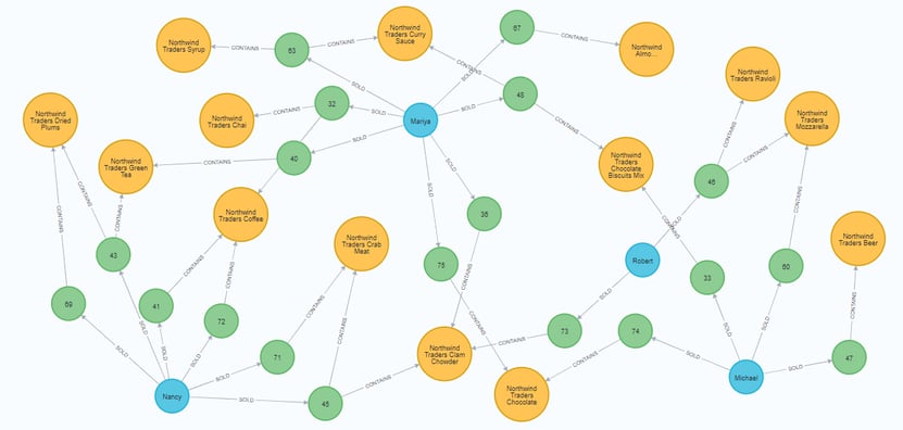
And if you run the following code block to get 30 nodes from the graph you can see the different relationships:
Cypher:
MATCH (n)-[]-(m) RETURN n, m LIMIT 30;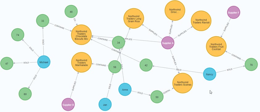
Next, you will query the resulting graph to find out what it can tell us about our newly-imported data.
Querying the Graph
Let's start with a couple of general queries to verify that our data matches the model we designed earlier in the guide. Here are some example queries.
Execute this cypher statement:
//find a sample of employees who sold orders with their ordered products
MATCH (e:Employee)-[rel:SOLD]->(o:Order)-[rel2:CONTAINS]->(p:Product)
RETURN e, rel, o, rel2, p LIMIT 25;
Results:

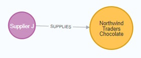
Execute this cypher statement:
//find the supplier and category for a specific product category
MATCH (s:Supplier)-[r1:SUPPLIES]->(p:Product {category: 'Candy'})
RETURN s, r1, p
Results:
Once you are comfortable that the data aligns with our data model and everything looks correct, you can start querying to gather information and insight for business decisions.
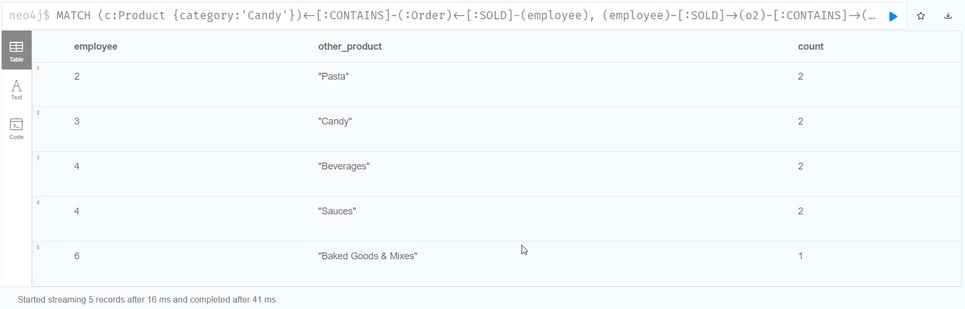
Which Employee had the Highest Cross-Selling Count of 'Candy' and Another Product?
Execute this cypher statement:
MATCH (c:Product {category:'Candy'})<-[:CONTAINS]-(:Order)<-[:SOLD]-(employee),
(employee)-[:SOLD]->(o2)-[:CONTAINS]->(other:Product)
RETURN employee.id as employee, other.category as other_product, count(distinct o2) as count
ORDER BY count DESC
LIMIT 5;
Looks like employee No. 4 was busy, though employee No. 2 also did well! Your results should look something like this:

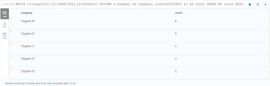
Which Suppliers supply the Highest Number of Products?
Execute this cypher statement:
MATCH (s:Supplier)-[r:SUPPLIES]-(p:Product)
RETURN s.company AS company, count(DISTINCT p) AS count
ORDER BY count DESC
LIMIT 5;
Your results should look something like this:

Want to find out more? Download our free Hop fact sheet now!


Blog comments